# Data Classification
When visualizing data for thematic maps, e.g. choropleth maps, the biggest task (at least for me) seems to be on how to organize the data used on the map to show a useful representation depicting the truth. This is to reveal patterns in the data set and create a sensible map. Similar values are grouped together and visualized accordingly to emphasize certain statements the map maker aims to visualize. With the data classification varibales, whether qualitative or quantitative, features are grouped together, that are alike. While doing so the map is being generalized. The following methods refer to quantitative data.
Histogram
When analizing the distribution of a data set a histogram is used to sort values into rank order. The x-axis depicts the range of possible values, the y-Axis shows the number of data records with these values. A look at the histogram can help with decisions about the number of classes, the method and more.
# Methods
There are different types of classifications that are highlighted below. To pick the right one for your data and map you need to take a look at the data, understand it and figure out what you want to say with your map. Characteristics of the data and the level of map generalization influence the decision for which method is used. Different classification methods for different data sets and different storys.
Classification Rules
Jenks & Coulson (1963) suggested 5 rules for data classification. Their rules state that data classification should meet the following requirements:
- Encompass the full range of the data.
- Have neither overlapping values nor vacant classes.
- Be great enough in number to avoid sacrificing the accuracy of the data, but not so numerous as to impute a greater degree of accuracy than is warranted bythe nature of the collected data.
- Divide the data into reasonably equal groups of observations.
- Have a logical mathematical relationship if practical.
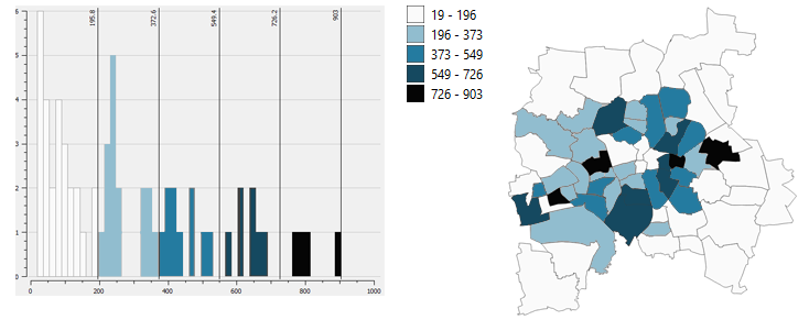
# Equal Interval Classification
Equal intervals group data defined by a specified data value. The intervals are equally spaced apart. This is especially useful for data that is distributed evenly. A nice legend with comprehensible values and simple class boundaries. If the data on the other hand is not distributed equally the classes can emphasize a biased interpretation of the data.
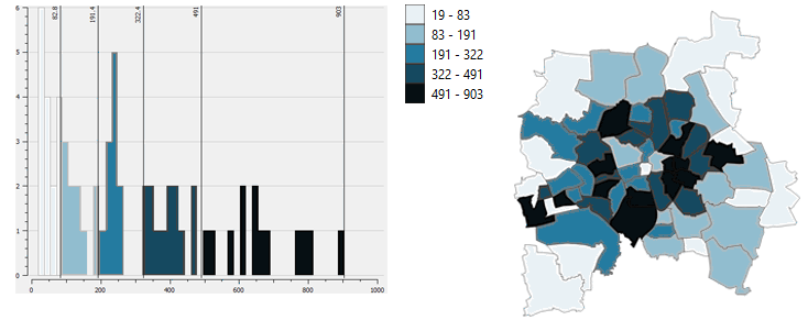
# Quantile Classification
When looking for break points that categorize the data equally in number, quantile classification is used for that. Each class includes the same amount of features. The data is sorted from lowest to highest based on a value and divide them into a number of classes. For example I have 150 data records and I want to group them into 5 classes. Therefore the lowest 30 features are categorized into the first quintile, the next 30 are grouped together into the second, and so on. Use cases include the emphatization of relative positions and exaggerate differences, such as income data. Difficulties with this method arise when features of a wide range are grouped together in a quantile minimizing their differences. The reverse case is possible, too: two similar values get grouped into different classes because they are close together but divided by a breaking point. Therefore the depiction of the data can indicate a significant difference between those values, when there is not.
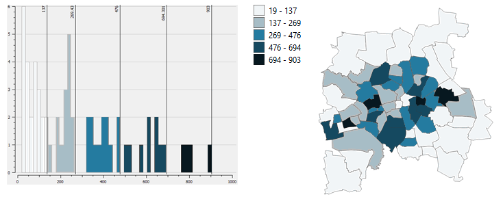
# Natural Breaks (Jenks)
The analyzation of data sets can reveal a pattern in the data distribution to reveal significant break points for natural groupings. Clumps of data are grouped together or spaces in the histogram break the data into groups. Mathmatical methods and complicated algorithms reveal such breaks and with the help of software (e.g. GIS) this can be easily done and is useful when data is not evenly distributed. It works well to represent such data but is not easily comprehensible by users as the classes do not have equal steps or equal amount of features, so that a manual revision could be needed to balance it out.
# Standard Deviation
Standard deviation is a number that states how far below or above a value is from the mean or average. Therefore not the definite value is used to be classified but a relative number and its multiple according to the value. The standard deviation classification method sorts the data based on this number for that distribution of data. It is useful for data with numerical values showing particular interests such as the distribution of income levels of areas to the average. The data for such should have a normal distribution, because outliers can skew the mean.
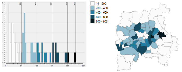
# Manual
There are situations where the breaks have to be set by the mapper.
TIP
Axis Maps (opens new window) list some good examples for such use cases:
- one class needs to be the mean
- a break needs to be set regardless
- the map is part of the series with the same range
- none of the methods above resemble the data close enough
# Number of Quantiles
How many classes are needed? How many are too much? With the number of classes the degree of map generalization is set: the more classes are used, the less generalization is happening, which is generally good, but mostly cause a confusing and too complex visualization. If too few quantiles are used, details are missed and the data is simplified, which might not be wanted.
As a rule of thumb myself, I mostly use 3 to 6 classes but it can vary depending on the data set. With too many classes it can be hard to distinguish the color or rather find a color range that is legible. I would use more classes for diverging ranges where I can use two different color ranges and therefore ensure legibility.
# Sturges' log function
Dent, Turguson & Hodler speak of Sturges' (1926) log function, that provides a good starting point to figure out the number of classes.
C ... number of classes
n ... number of observations/data records
# Terms of Quantiles
| Number of Quantiles | Name |
|---|---|
| 2 | Median |
| 3 | Tertile |
| 4 | Quartile |
| 5 | Quintile |
| 10 | Decitile |
| 100 | Percentile |
# References
- Axis Maps. Basics of Data Classification (opens new window) (accessed 6 Jun 2020).
- Boyes, D. Data classification methods for mapping (opens new window) (accessed 6 Jun 2020).
- Dent, B. D., Torguson, J. S. & Hodler, T. W., 2009. Cartography - Thematic Map Design. 6th Edition ed. New York: McGraw-Hill.
- Jenks, G. F. & Coulson, M. R. C., 1963. Class Intervals for Statistical Maps, International Yearbook of Cartography, Vol. III, p. 120.
- Robinson, A. C. Data Classification - Breaking Up Is Hard To Do (opens new window) (accessed 6 Jun 2020).